Measure What Matters: Finding the Best Radiological Anomaly Localisation Model
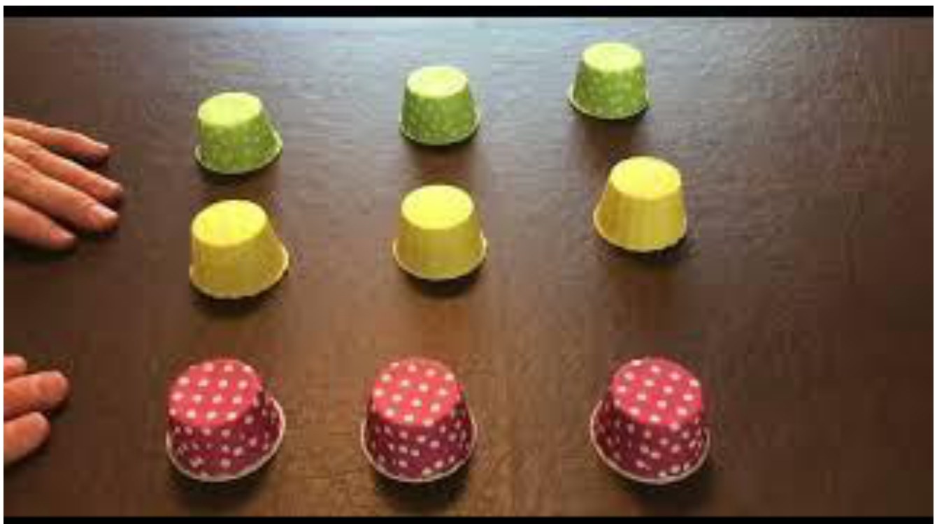
Three red cups, a piece of candy, and a pair of hands shuffling them around. Follow the cup and you will know where the candy is. Now rewind the video: did you notice that the cups changed colour halfway through? That a third pair of hands appeared? Most people track the cup perfectly and miss everything else. Attention is a spotlight, and a spotlight has an edge: whatever falls outside it is simply not seen.
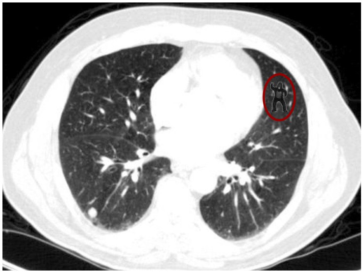
This is not a curiosity of party tricks. When Drew, Vo and Wolfe rendered a gorilla into a lung CT and asked trained radiologists to count lung nodules, more than 50% of the experts missed the gorilla entirely. Inattentional blindness does not care about expertise. If anything, expertise makes it worse: the more efficient your search strategy, the tighter the spotlight.
Which raises an obvious question. Could a machine be the second pair of eyes that never gets bored, never gets a search template stuck in its head, and flags the thing nobody was looking for?
That question has driven most of my work for the last years. And the longer I work on it, the clearer it becomes that the hard part is not the model. The hard part is measuring what we actually want.
The system we want to build
The vision is simple. Take a volumetric scan, run it through a model, and highlight everything that deviates from normal - not just the pathology you were told to look for. A tumor, a stroke, a handful of tiny lesions, a hidden shape, a subtle discolouration that only shows up in two slices, a structure that should be there and is not. Then let the radiologist's attention do what it does well, focused by the model's flags.
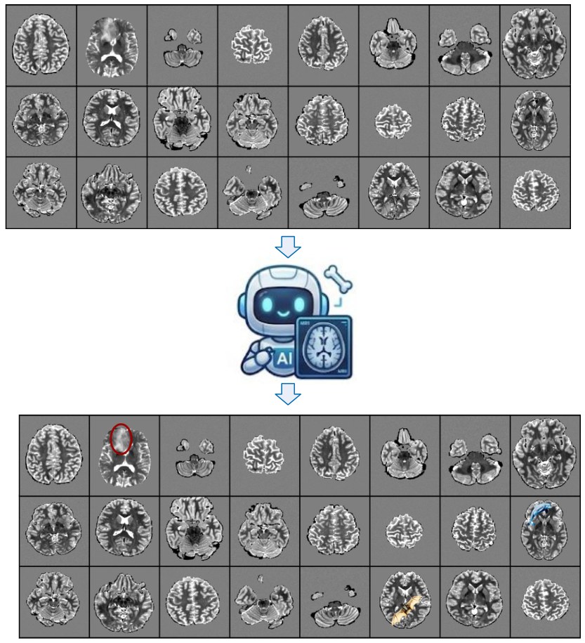
Note what makes this different from a standard segmentation network. We never say "find the lung nodule". We say: here is what healthy looks like - show me everything that does not fit. That is unsupervised anomaly detection, and it is attractive precisely because it does not need labels for the disease. Rare findings, unknown conditions, novel scanners: in principle, all of it is covered by a single definition of normal.
In practice, "everything that does not fit" is a much harder promise than it sounds.
What does abnormal even mean?
Normality, in this setting, is defined by the training data - not by a rule book. Show the model a set of normal samples, and it learns what normal is.
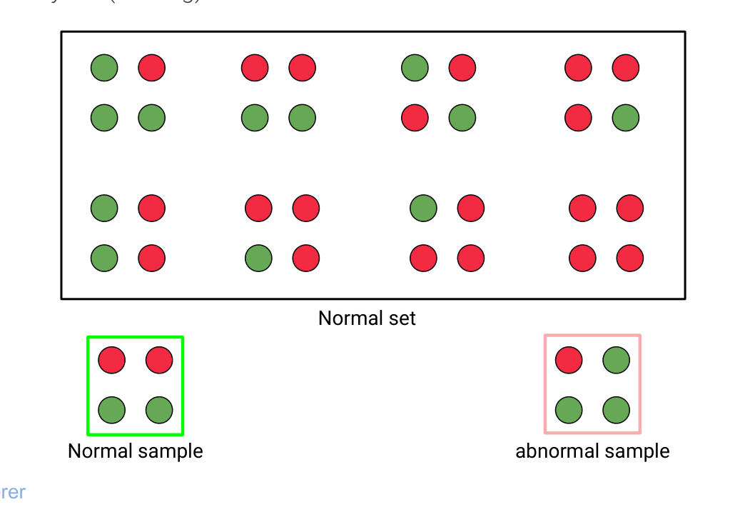
In a toy problem this is easy - every normal sample has a red dot in the top-right corner, so anything without one is abnormal. Real data is never that clean. We only ever have a limited sample of normality, so we have to model the underlying distribution and hope the model matches reality.
And here the trouble starts. Several different models can explain the same limited data equally well - different assumptions, different architectures, different regularisation. Feed them new points and they disagree, especially about the points that matter most: the borderline ones.
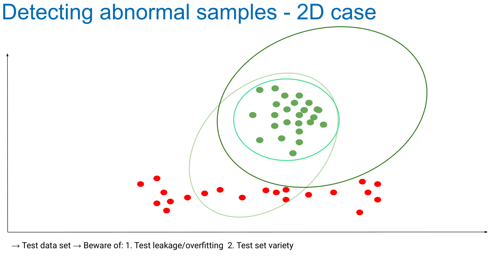
This is why test data is so dangerous in this field. If we tune our model while looking at the test set, we are not measuring generalisation - we are measuring how well we fit the test set. And if the test set only contains the anomalies we already have labels for, it will never tell us whether the model can catch the unexpected. A model trained and tested on lung nodules will not suddenly find the gorilla.
In medical imaging, there is an additional twist: we do not just want to know if a volume is abnormal, we want to know where - the pathology needs to be localized for the heatmap to be useful at all. So the problem is really anomaly localization: fit a model of normal anatomy, and then map every deviation from it.
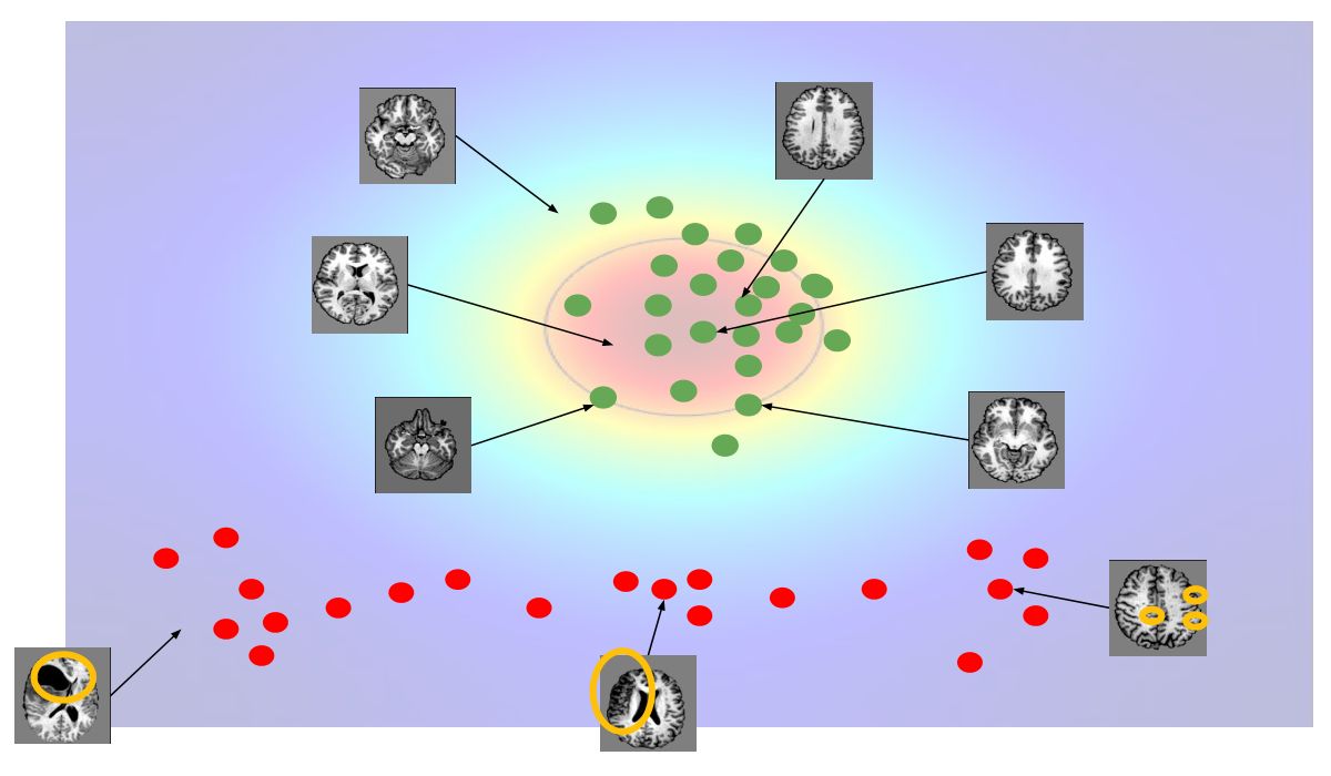
The tempting shortcut is familiar: pick a model off the shelf, train it on whatever data is lying around, watch it look reasonable on a handful of examples, and start talking about deployment. Reality hits immediately - and it hits in three places: the data, the findings, and the metrics.
Reality check 1: the data is nothing like ImageNet
Medical volumes break most of the assumptions that make modern deep learning work.
| Property | Natural images / benchmarks | Medical volumes |
|---|---|---|
| Sample size | a few megapixels | \(256^3\) to \(512^3\) voxels |
| Dataset size | millions of samples | ~1,000 samples is already large |
| Heterogeneity | curated, homogeneous | scanners, protocols, artifacts, preprocessing |
| Pretraining | ImageNet, CLIP, … | no general-purpose backbone for most modalities |
Every dimension hurts. Volumes are enormous, datasets are tiny, and the data is heterogeneous in ways that are invisible until you look at it. Add the clinical reality - motion, noise, reconstruction artifacts, missing anatomy, different protocols - and the beautifully preprocessed datasets from the papers start looking like a different world.
"Just make the 2D network 3D" is a one-line change in most frameworks, and it even works reasonably well on clean benchmarks. But no amount of network surgery fixes a missing pretrained encoder, and none of it prepares you for what the data actually looks like in a hospital.
Reality check 2: the obvious anomaly is the one you don't need to find
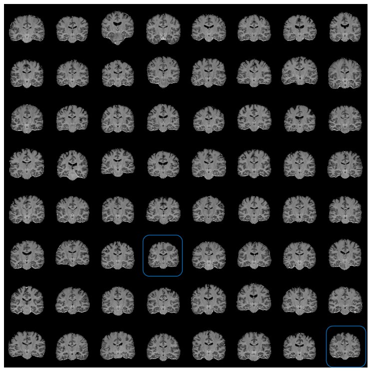
Here is a test that changed how I look at heatmaps. Given the scans below, which findings do you notice?
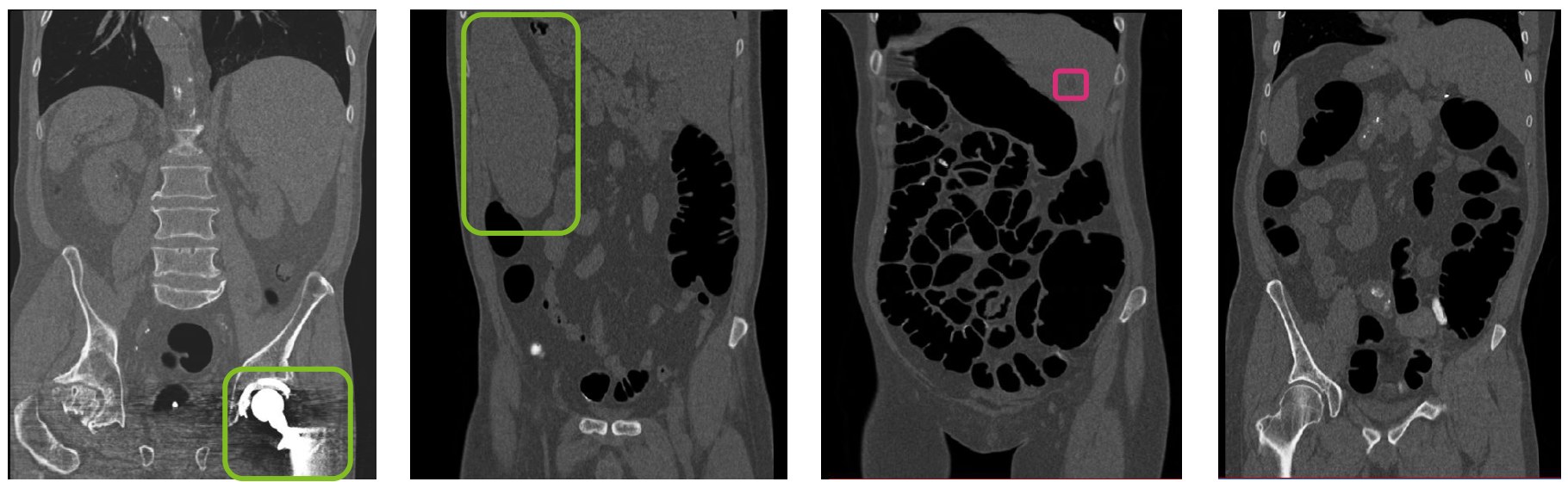
Two algorithms are competing. One lights up the big, obvious structures - the implant, the spleen. The other is easy to miss while scrolling, but it catches the subtle little thing. Intuitively, the first one looks better. Clinically, it is almost worthless: the large, conspicuous findings are found by the radiologist in two seconds anyway. The subtle findings - the low-contrast lesion that shows up on three or four slices before vanishing, the organ that is simply absent - are exactly the ones that get overlooked, and often the small and inconspicuous anomalies are the most relevant and most helpful ones in practice.
In a large screening programme this becomes a needle-in-a-haystack problem. Thousands of scans, a handful of actionable findings, and a metric that will happily reward you for re-detecting the implant every time.
What happened when we went "in the wild"
I wanted to know how this plays out at population scale, so we took a 3D context-encoding VAE (ceVAE) - a model that had performed well on curated brain benchmarks - and evaluated it on a large-scale population study of 10,000 participants with T1-weighted and FLAIR brain scans. Unlike the usual setup, the cohort was representatively sampled and contained the full variety of incidental findings (refIFs), not one clean pathology.
On the classic segmentation numbers, everything looked fine:
| Metric (dataset level, refIF scans) | Value |
|---|---|
| AUROC | 0.838 |
| AP | 0.312 |
| Dice | 0.382 |
For orientation: the same model on the well-curated BraTS17 benchmark reached AUROC 0.934 and AP 0.24, so 0.838/0.312 did not set off any alarms. But those numbers were computed the usual way - all pixels of all scans pooled into one bucket, the so-called dataset level. When we computed the score per scan and averaged, the picture collapsed:
| Metric | Dataset level | Aggregated per scan |
|---|---|---|
| Dice | 0.382 | 0.061 |
| AP | 0.312 | 0.108 |
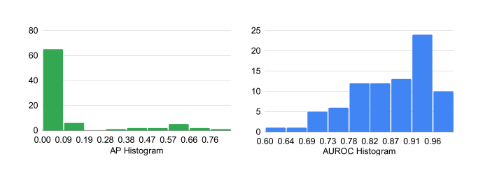
A six-fold drop that nobody would have noticed from the headline number. The dataset-level score was being carried by a handful of large, easy-to-detect anomalies, while for most scans the algorithm simply failed. The metric was dominated by exactly the findings that needed the least help.
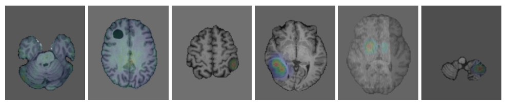
To find out what was really going on, we had an expert radiologist review every prediction above the detection threshold. The algorithm flagged 83 suspicious regions across the cohort, which the radiologist sorted into false positives, brain-extraction failures, imaging artifacts, not-medically-relevant anomalies, and genuine incidental findings - the first two counting as algorithm failures, the last three as correct detections.
Against 84 reference incidental findings, the outcome was sobering:
- 19 of 84 reference findings were detected - and 16 of those 19 were grade C1 ("very conspicuous, should definitely be found").
- Still, 21 of 37 (>50%) of the C1 findings were missed.
- Detection quality collapsed with conspicuity:
| Conspicuity grade | Detected | Reference |
|---|---|---|
| C1 - very conspicuous | 16 | 37 |
| C2 - partially conspicuous | 3 | 39 |
| C3 - unobtrusive | 0 | 8 |
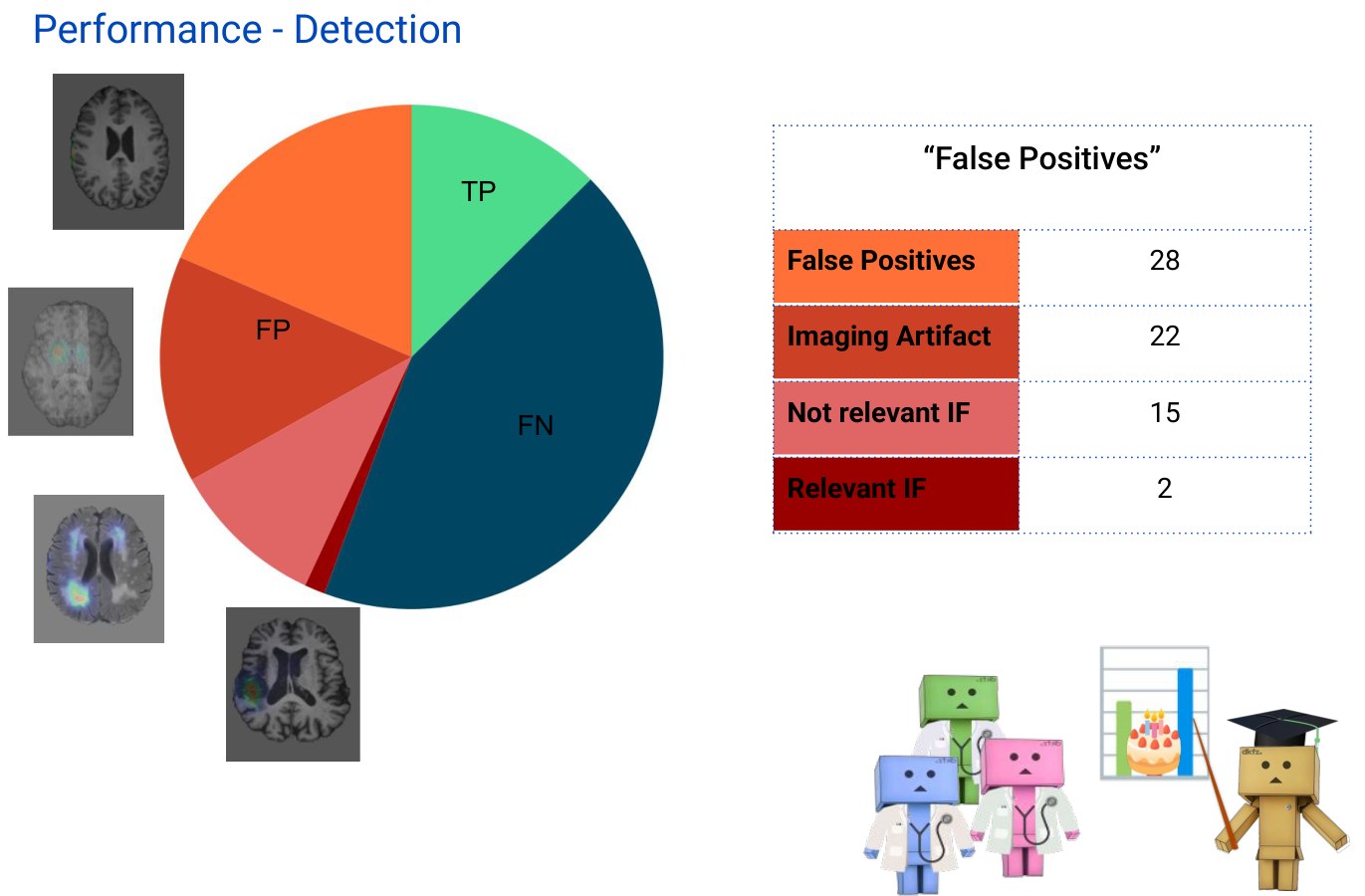
Put bluntly: the system reliably found image corruptions and large anomalies and essentially nothing else. Neither precision nor recall was good enough for day-to-day clinical use.
But it was not useless. The algorithm surfaced 31 anomalies that had not been reported previously - 22 in the test set, 2 in validation, and 7 in the training set. The last number is its own quiet warning: even carefully curated "normal" training data contains unreported pathology, and a model that learns from it will learn the wrong definition of normal. And even when the specific detection is wrong, flagging that a scan contains out-of-distribution content at all is valuable as a pre-filter - a safety net for fully automated pipelines and large screening programmes.
The deepest lesson was not about the model. It was this:
Our metric was optimising pixel overlap. Our clinical objective was to surface the inconspicuous finding. The alignment between the medical objective and the metric was simply wrong.
Measuring what matters
That mismatch is what turned me into a metrics person. Consider this innocent-looking quiz. Below, the reference has three structures. Prediction 1 finds one of them but segments it beautifully. Prediction 2 finds all three, slightly less precisely per-structure.
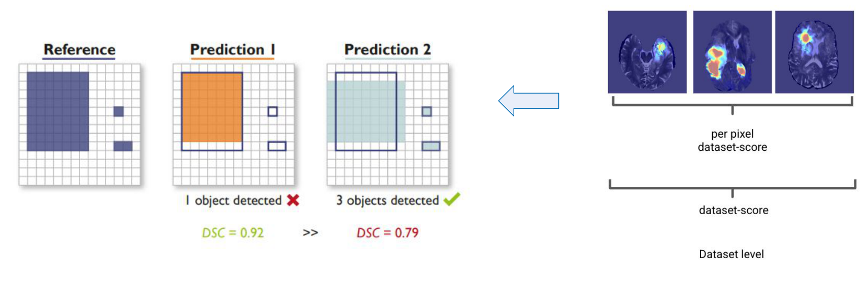
Dice picks Prediction 1. Any radiologist picks Prediction 2. This is not a corner case - it is the default outcome whenever segmentation metrics meet anomaly localization, and it is why the field needed to look at its metrics from scratch.
In Beyond Heatmaps we did exactly that: we revisited the anomaly localization setup, analysed the metrics it has borrowed from neighbouring fields, and compared them under controlled conditions and against human judgement.
Four levels of evaluation
Before picking a metric, decide what you are aggregating over:
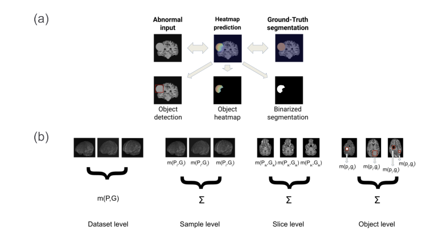
- Dataset level - pool all pixels of all scans, compute one score. Broad, but large objects dominate.
- Sample level - one score per scan, then average. The segmentation convention; silently ignores whether objects were missed.
- Slice level - one score per 2D slice. Cheap, matches 2D models, but blind to 3D structure.
- Object level - one score per distinct anomaly (via connected components), then aggregate. Fixes the size bias, but can ignore normal scans.
The choice is not cosmetic. In the population study above, dataset level said Dice 0.38; sample level said 0.06.
The metric families
Segmentation metrics (DSC, IoU) measure overlap - but they need a binarisation threshold, and the best-threshold variant is the usual workaround:
Ranking / out-of-distribution metrics (AUROC, AP) consume the heatmap directly, without thresholding:
Object-detection and instance-segmentation metrics move the unit of evaluation from pixels to objects: Instance IoU per object, or the center-point distance between predicted and true centres of mass:
A simple, robust variant is center matching: a predicted heatmap centre that falls inside the convex hull of a labelled object counts as a hit. From hits, misses, and false detections you can compute \(F_1\), precision, and recall at the object level - much closer to how a reader judges a heatmap.
And the anomaly-localization metric we proposed, SoftInstanceIoU. It evaluates each object against the continuous prediction and explicitly scores the background, so it needs no binarisation threshold:
The background term (target 0, weighted by \(\alpha\)) is what makes a "fire-everywhere" model pay for its false positives.
Why the borrowed metrics fail
The fundamental problem is that anomaly detection is not segmentation. Many scans are completely normal: no ground-truth objects, no predictions, nothing to overlap. Mathematically, DSC, IoU, AP and AUROC are all undefined when there is only one class.
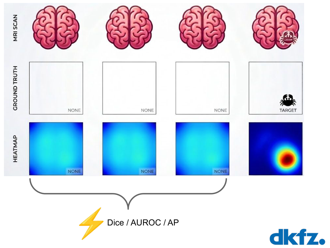
The community's usual fix is to pool everything at dataset level - which is how we ended up in the population-study trap. SoftInstanceIoU and object-level \(F_1\) avoid that trade-off: they are defined on normal scans, they score background explicitly, and they treat each anomaly as an individual, so a large lesion can no longer outvote three small ones.
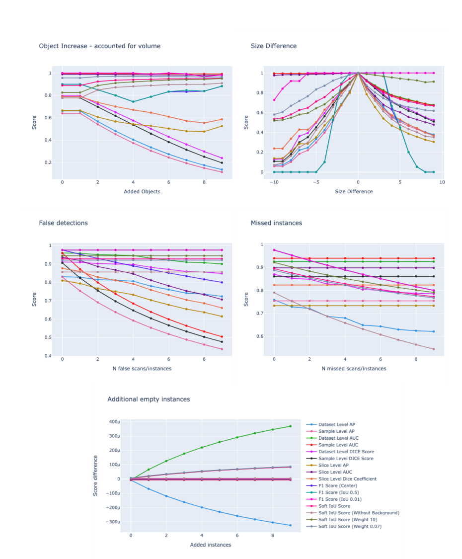
Do the numbers agree with the humans?
Metrics are only meaningful if they track the judgement of the people who use them. We had an expert review per-object predictions from seven algorithms on CamCAN (with injected artificial anomalies) and the winning entries of the MOOD brain and abdominal challenges - blinded to which method produced which heatmap.
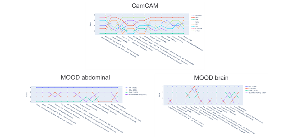
Object-based metrics come with two more gifts. Their ranking is stable under bootstrapping - we can show that the ordering of methods is not an artifact of one lucky test set. And because every object gets a continuous score, we can sort them into an AUROC-like curve: the leading portion reflects background segmentation quality, the tail exposes poorly detected and entirely missed objects. One plot, the whole distribution of performance - far more informative than a single pooled number.
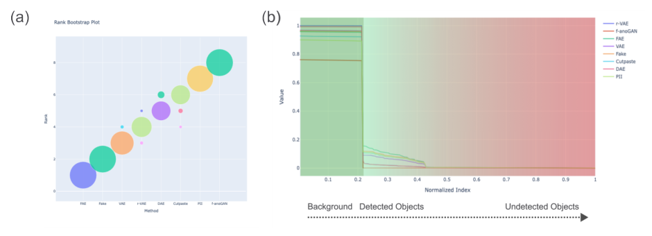
Bottom line: the right metric is use-case dependent, but SoftInstanceIoU and other object-based metrics show significant promise - resilient to false positives while still sensitive to missed detections. Exactly the trade-off that clinical anomaly detection needs.
A fair fight: the MOOD benchmark
Good metrics only help if everyone is measuring under the same, honest conditions. That is what the Medical OOD Detection Benchmark (MOOD) provides - an international MICCAI challenge that ran from 2020 to 2025:
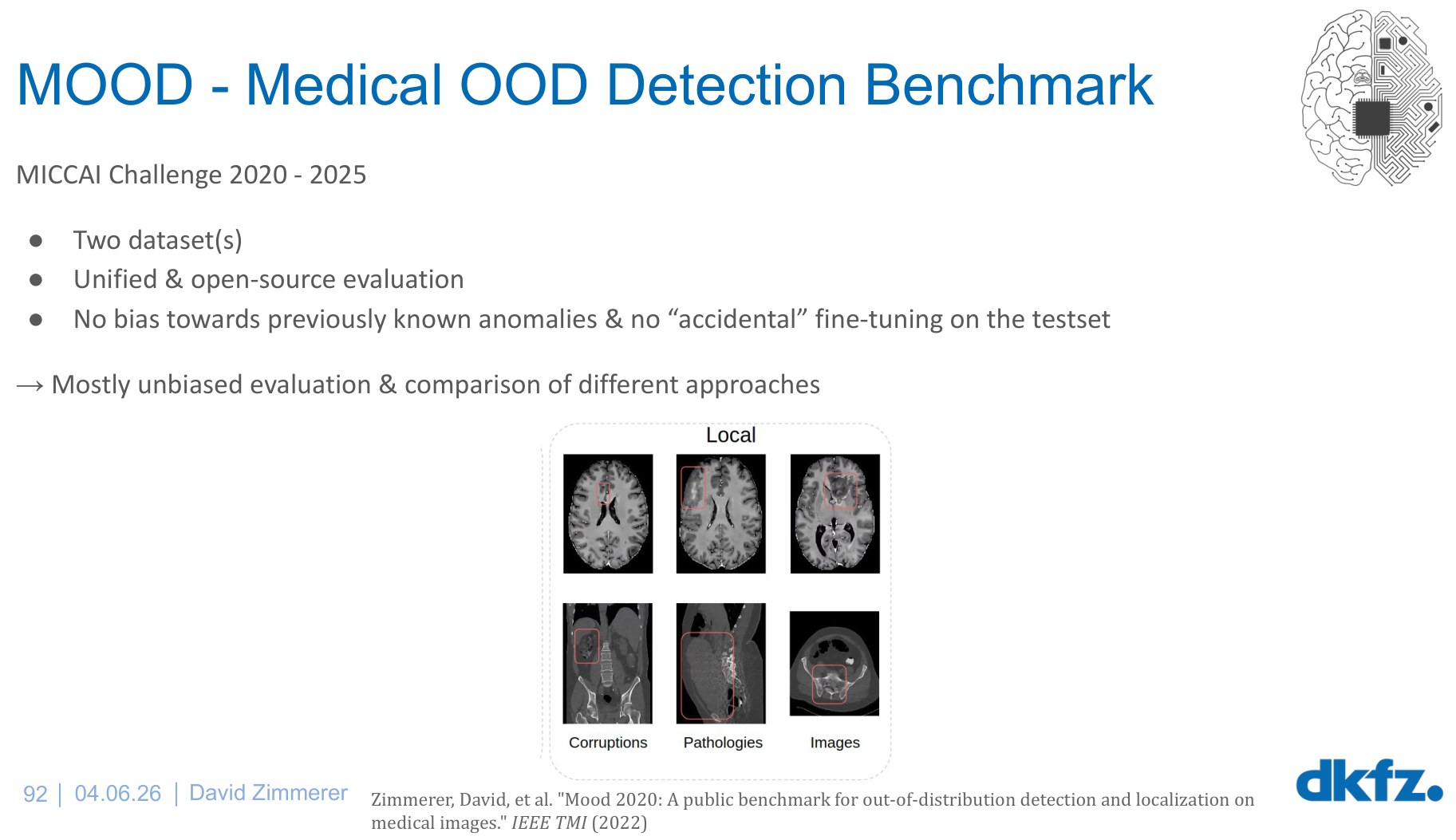
- Two datasets (brain MRI and abdominal CT), so methods must generalise across anatomies instead of tuning to one.
- Unified, open-source evaluation, with Docker-based submission on a hidden test set - no test leakage, no accidental fine-tuning, no leaderboard overfitting.
- No bias towards previously known anomalies. Participants do not know what to expect; the test set even contains rendered gorillas, testing whether a method generalises to genuinely unexpected content.
The result is a mostly unbiased comparison - the closest thing our field has to a
clean playing field. And in the spirit of open science, the datasets are publicly
available (mood_brain,
mood_brain_test).
What actually works
Benchmarks also let us see which method families hold up in practice.
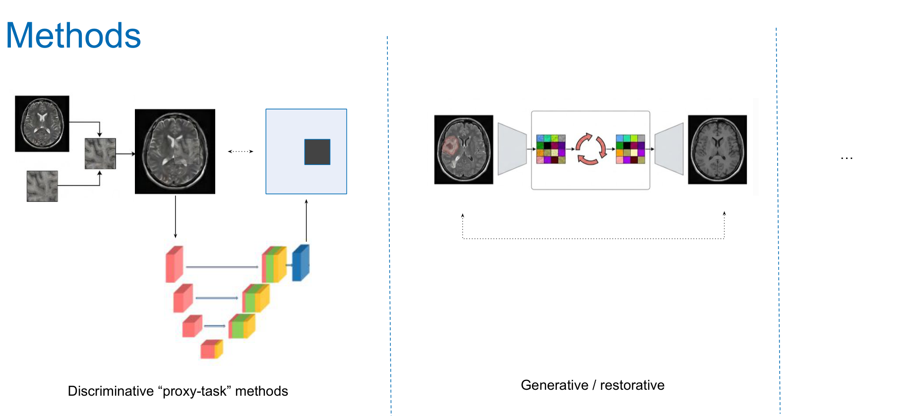
Discriminative "proxy-task" methods. Take normal images, inject synthetic objects - interpolated foreign patches, blobs, Gaussian noise - and train a network to segment only the injected object. At test time you hope the network generalises from synthetic to real anomalies. Foreign Patch Interpolation is the best-known instance, and it has proven remarkably strong: not only on our test set, but across many methods and datasets.
Generative / restorative methods. Train a model to reconstruct normal data only. Feed it an abnormal scan, and compare input and reconstruction: the model, having never seen pathology, "heals" the anomaly, and the residual localises it.
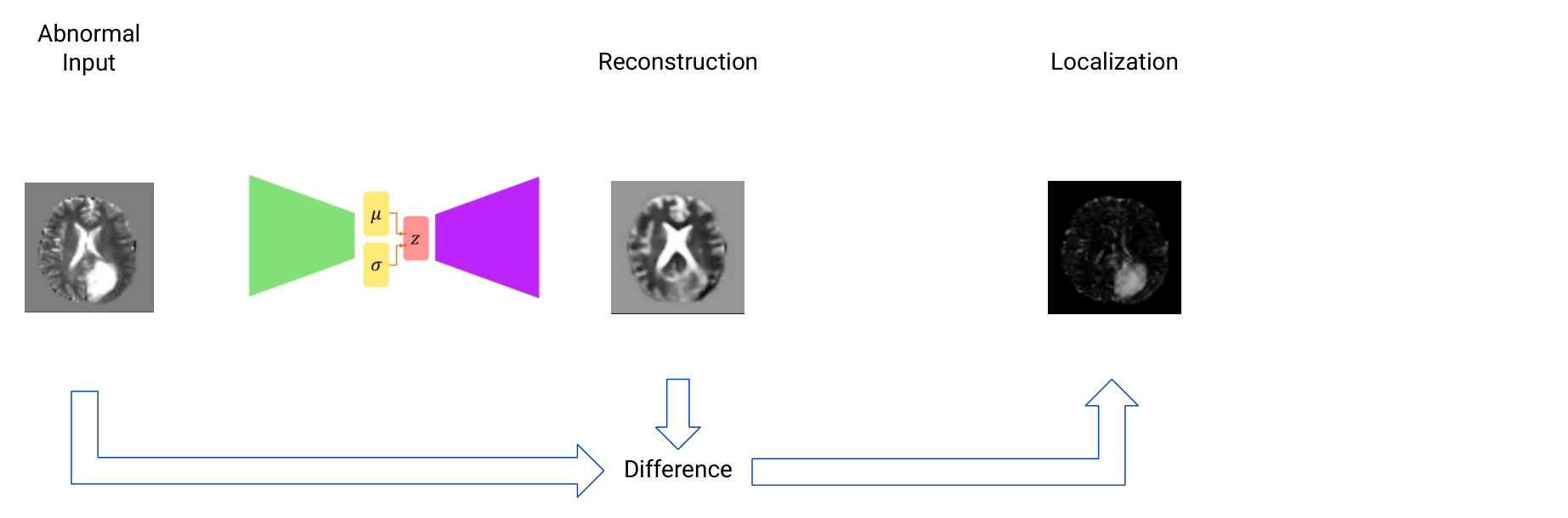
Autoencoders were the starting point; diffusion models are the state of the art today, with markedly better reconstructions. There is also an elegant alternative view: a generative model with an explicit likelihood exposes the score - the gradient of the log-likelihood with respect to the image - which points toward normality and highlights the abnormal region directly. And while most of the field races to reduce false positives, I keep wondering whether that is the right target, given that missed instances are the clinically expensive error.
Feature-bank and distillation / teacher-student methods dominate on natural images: store features of normal data and use \(k\)-nearest-neighbours for local density estimation, or train a student to diverge from a teacher on anomalies. For medical imaging, they share one blocker: they need pretrained feature encoders, and no robust, general-purpose medical backbone covers all organs, modalities, and resolutions yet. Building those backbones is one of the open frontiers this field still owes itself.
The final frontier: context
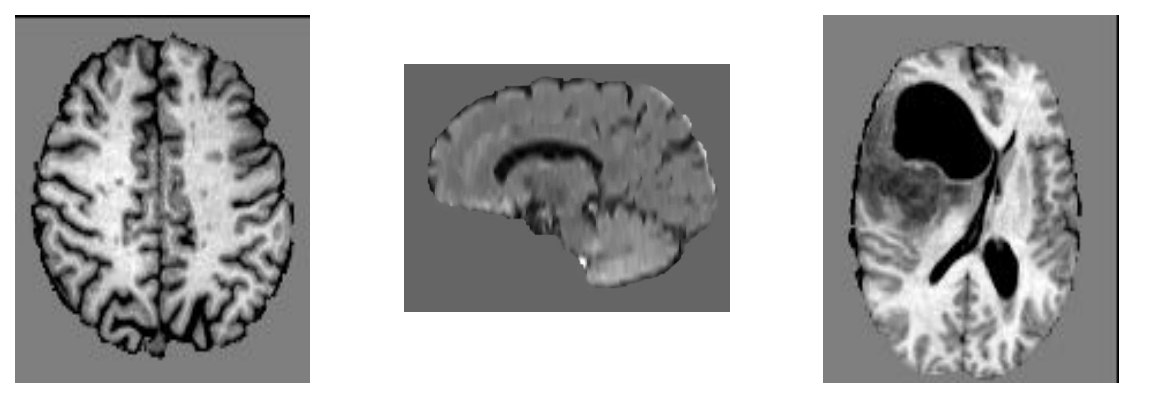
One last quiz. Five brain slices; which one is abnormal?
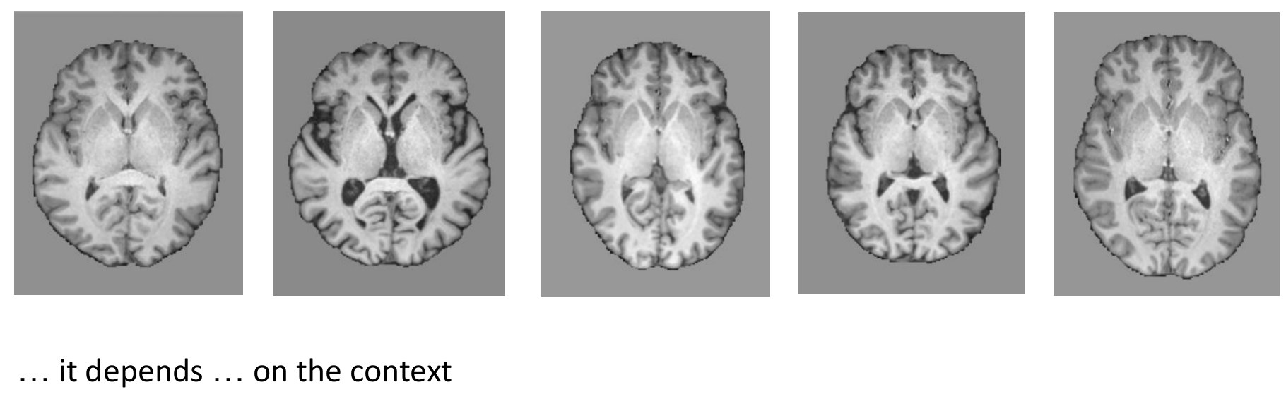
The answer is "it depends - on the context". The same image is normal in one patient and pathological in another, and the deciding information - age, sex, history, protocol - is often not in the image at all. No anomaly detector trained on pixels alone can resolve this, and no metric that scores a heatmap in isolation can reward getting it right.
That, to me, is the boundary where anomaly detection stops being a computer vision problem and becomes a clinical one. It is also where the next generation of evaluation has to go: from "is this pixel abnormal?" to "is this finding abnormal for this patient?"
What I take away
- The gorilla is real. Expertise does not protect against inattentional blindness. The most valuable anomaly is often the one nobody was looking for - small, low-contrast, inconspicuous, unlabelled.
- Segmentation metrics lie in this setting. They are undefined on normal scans, and when pooled at dataset level they reward large, easy findings. In the wild, dataset Dice 0.38 became per-scan Dice 0.06.
- What you measure decides what you optimise. Object-level, threshold-insensitive metrics - above all SoftInstanceIoU - best match human judgement and correctly reward finding all anomalies, including the small ones.
- Honest benchmarks require adversarial design. Hidden test sets, Docker-based evaluation, multiple anatomies, and unexpected anomalies are what separate real generalisation from leaderboard overfitting.
- Methods are improving, but context is unsolved. Proxy-task and restorative methods - especially diffusion-based ones - lead the pack; pretrained-encoder methods are blocked on missing medical backbones; and no heatmap knows how old the patient is.
If we want AI to be the second pair of eyes that catches the unexpected, we have to stop measuring the easy things first. Measure what matters.
References
- Drew, T., Vo, M. L.-H., Wolfe, J. M. The invisible gorilla strikes again: sustained inattentional blindness in expert observers. Psychological Science, 2013.
- Zimmerer, D., Maier-Hein, K. Beyond Heatmaps: A Comparative Analysis of Metrics for Anomaly Localization in Medical Images. UNSURE, 2024.
- Zimmerer, D., Paech, D., Lüth, C., Petersen, J., Köhler, G., Maier-Hein, K. Unsupervised Anomaly Detection in the Wild. BVM, 2022.
- Zimmerer, D., Full, P. M., Isensee, F., et al. MOOD 2020: A Public Benchmark for Out-of-Distribution Detection and Localization on Medical Images. IEEE TMI, 2022.
- Tan, J., Hou, B., Batten, J., Qiu, H., Kainz, B. Detecting Outliers with Foreign Patch Interpolation. arXiv:2011.04197, 2020.
- Behrendt, F., et al. Guided Reconstruction with Conditioned Diffusion Models for Unsupervised Anomaly Detection in Brain MRIs. Computers in Biology and Medicine, 2025.
- Reinke, A., et al. Common Limitations of Image Processing Metrics: A Picture Story. arXiv:2104.05642, 2021.
- Maier-Hein, L., et al. Metrics Reloaded: Recommendations for Image Analysis Validation. arXiv:2206.01653, 2023.